Arduino Mega 2560 pin map

ATmega2560-Arduino Pin Mapping

Below is the pin mapping for the Atmega2560. The chip used in Arduino 2560. There are pin mappings to Atmega8 and Atmega 168/328 as well.

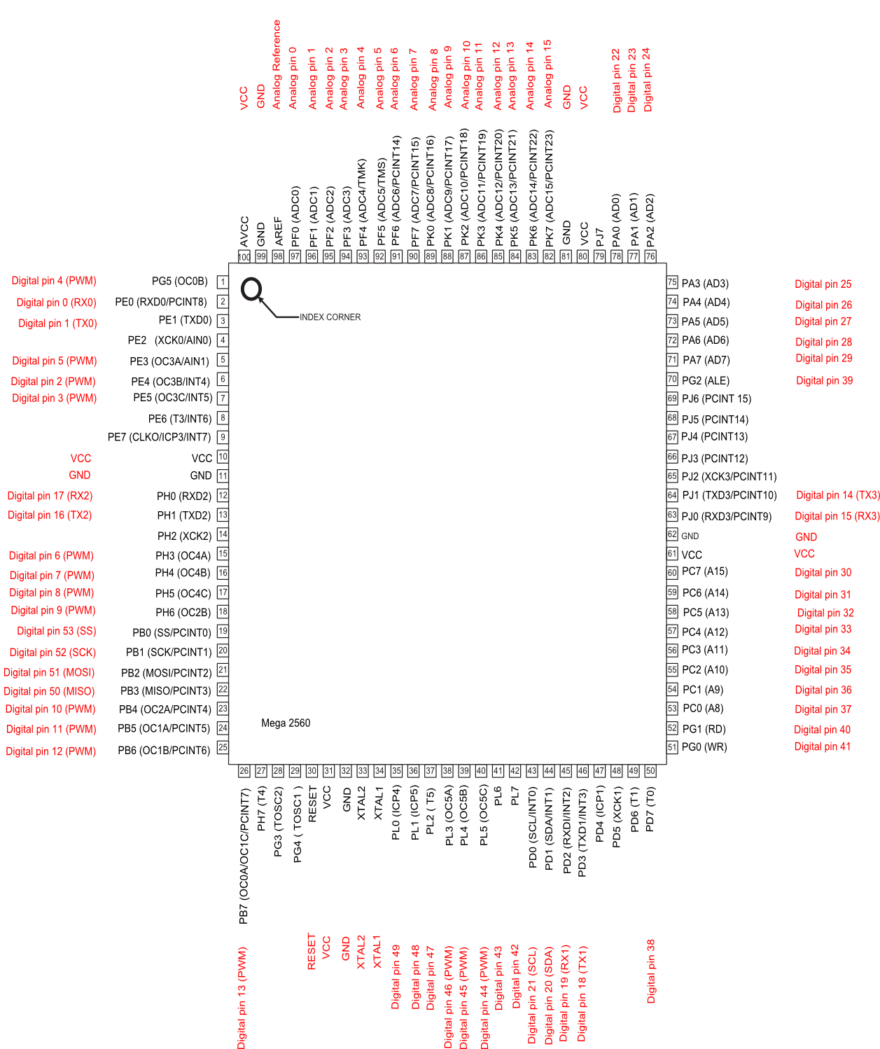
Arduino Mega 2560 PIN diagram

The source SVG file is also available for download: PinMapping2560.zip

Arduino Mega 2560 PIN mapping table

Pin Number	Pin Name	Mapped Pin Name
1	PG5 ( OC0B )	Digital pin 4 (PWM)
2	PE0 ( RXD0/PCINT8 )	Digital pin 0 (RX0)
3	PE1 ( TXD0 )	Digital pin 1 (TX0)
4	PE2 ( XCK0/AIN0 )
5	PE3 ( OC3A/AIN1 )	Digital pin 5 (PWM)
6	PE4 ( OC3B/INT4 )	Digital pin 2 (PWM)
7	PE5 ( OC3C/INT5 )	Digital pin 3 (PWM)
8	PE6 ( T3/INT6 )
9	PE7 ( CLKO/ICP3/INT7 )
10	VCC	VCC
11	GND	GND
12	PH0 ( RXD2 )	Digital pin 17 (RX2)
13	PH1 ( TXD2 )	Digital pin 16 (TX2)
14	PH2 ( XCK2 )
15	PH3 ( OC4A )	Digital pin 6 (PWM)
16	PH4 ( OC4B )	Digital pin 7 (PWM)
17	PH5 ( OC4C )	Digital pin 8 (PWM)
18	PH6 ( OC2B )	Digital pin 9 (PWM)
19	PB0 ( SS/PCINT0 )	Digital pin 53 (SS)
20	PB1 ( SCK/PCINT1 )	Digital pin 52 (SCK)
21	PB2 ( MOSI/PCINT2 )	Digital pin 51 (MOSI)
22	PB3 ( MISO/PCINT3 )	Digital pin 50 (MISO)
23	PB4 ( OC2A/PCINT4 )	Digital pin 10 (PWM)
24	PB5 ( OC1A/PCINT5 )	Digital pin 11 (PWM)
25	PB6 ( OC1B/PCINT6 )	Digital pin 12 (PWM)
26	PB7 ( OC0A/OC1C/PCINT7 )	Digital pin 13 (PWM)
27	PH7 ( T4 )
28	PG3 ( TOSC2 )
29	PG4 ( TOSC1 )
30	RESET	RESET
31	VCC	VCC
32	GND	GND
33	XTAL2	XTAL2
34	XTAL1	XTAL1
35	PL0 ( ICP4 )	Digital pin 49
36	PL1 ( ICP5 )	Digital pin 48
37	PL2 ( T5 )	Digital pin 47
38	PL3 ( OC5A )	Digital pin 46 (PWM)
39	PL4 ( OC5B )	Digital pin 45 (PWM)
40	PL5 ( OC5C )	Digital pin 44 (PWM)
41	PL6	Digital pin 43
42	PL7	Digital pin 42
43	PD0 ( SCL/INT0 )	Digital pin 21 (SCL)
44	PD1 ( SDA/INT1 )	Digital pin 20 (SDA)
45	PD2 ( RXDI/INT2 )	Digital pin 19 (RX1)
46	PD3 ( TXD1/INT3 )	Digital pin 18 (TX1)
47	PD4 ( ICP1 )
48	PD5 ( XCK1 )
49	PD6 ( T1 )
50	PD7 ( T0 )	Digital pin 38
51	PG0 ( WR )	Digital pin 41
52	PG1 ( RD )	Digital pin 40
53	PC0 ( A8 )	Digital pin 37
54	PC1 ( A9 )	Digital pin 36
55	PC2 ( A10 )	Digital pin 35
56	PC3 ( A11 )	Digital pin 34
57	PC4 ( A12 )	Digital pin 33
58	PC5 ( A13 )	Digital pin 32
59	PC6 ( A14 )	Digital pin 31
60	PC7 ( A15 )	Digital pin 30
61	VCC	VCC
62	GND	GND
63	PJ0 ( RXD3/PCINT9 )	Digital pin 15 (RX3)
64	PJ1 ( TXD3/PCINT10 )	Digital pin 14 (TX3)
65	PJ2 ( XCK3/PCINT11 )
66	PJ3 ( PCINT12 )
67	PJ4 ( PCINT13 )
68	PJ5 ( PCINT14 )
69	PJ6 ( PCINT 15 )
70	PG2 ( ALE )	Digital pin 39
71	PA7 ( AD7 )	Digital pin 29
72	PA6 ( AD6 )	Digital pin 28
73	PA5 ( AD5 )	Digital pin 27
74	PA4 ( AD4 )	Digital pin 26
75	PA3 ( AD3 )	Digital pin 25
76	PA2 ( AD2 )	Digital pin 24
77	PA1 ( AD1 )	Digital pin 23
78	PA0 ( AD0 )	Digital pin 22
79	PJ7
80	VCC	VCC
81	GND	GND
82	PK7 ( ADC15/PCINT23 )	Analog pin 15
83	PK6 ( ADC14/PCINT22 )	Analog pin 14
84	PK5 ( ADC13/PCINT21 )	Analog pin 13
85	PK4 ( ADC12/PCINT20 )	Analog pin 12
86	PK3 ( ADC11/PCINT19 )	Analog pin 11
87	PK2 ( ADC10/PCINT18 )	Analog pin 10
88	PK1 ( ADC9/PCINT17 )	Analog pin 9
89	PK0 ( ADC8/PCINT16 )	Analog pin 8
90	PF7 ( ADC7 )	Analog pin 7
91	PF6 ( ADC6 )	Analog pin 6
92	PF5 ( ADC5/TMS )	Analog pin 5
93	PF4 ( ADC4/TMK )	Analog pin 4
94	PF3 ( ADC3 )	Analog pin 3
95	PF2 ( ADC2 )	Analog pin 2
96	PF1 ( ADC1 )	Analog pin 1
97	PF0 ( ADC0 )	Analog pin 0
98	AREF	Analog Reference
99	GND	GND
100

rfcomm server example c linux

$ gcc rfcomm-server.c -lbluetooth
$ ./a.out


#include
#include
#include
#include
#include

int main(int argc, char **argv)
{
    struct sockaddr_rc loc_addr = { 0 }, rem_addr = { 0 };
    char buf[1024] = { 0 };
    int s, client, bytes_read;
    socklen_t opt = sizeof(rem_addr);

    // allocate socket
    s = socket(AF_BLUETOOTH, SOCK_STREAM, BTPROTO_RFCOMM);

    // bind socket to port 1 of the first available
    // local bluetooth adapter
    loc_addr.rc_family = AF_BLUETOOTH;
    loc_addr.rc_bdaddr = *BDADDR_ANY;
    loc_addr.rc_channel = (uint8_t) 15;
    bind(s, (struct sockaddr *)&loc_addr, sizeof(loc_addr));

    // put socket into listening mode
    listen(s, 1);
    client=0;    // initialize connection handle.
    while(1)
    {  
            if( client == 0 )
            {
            // accept one connection
            printf("accept wait\n");
            client = accept(s, (struct sockaddr *)&rem_addr, &opt);
            printf("now accept %d\n",client);
 
            ba2str( &rem_addr.rc_bdaddr, buf );
            fprintf(stderr, "accepted connection from %s\n", buf);
            memset(buf, 0, sizeof(buf));
            }
 
            // read data from the client
            bytes_read = read(client, buf, sizeof(buf));
            if( bytes_read > 0 )
            {
                printf("received [%s]\n", buf);
            }
            else
            if( bytes_read < 0 )
            {
                close(client);
                client=0;
                printf("close connection\n");
            }
            printf("bytes_read [%d]\n",bytes_read);
    }

    // close connection
    close(client);
    close(s);
    return 0;
}

Bitwise Tips and Tricks - From

Below from http://www.opensourceforu.com/2012/06/power-programming-bitwise-tips-tricks/

Bitwise Tips and Tricks

By Balbir Singh on June 27, 2012 in Coding, Developers · 0 Comments

If you are a seasoned programmer, these tips and tricks will seem very familiar, and are probably already part of your repertoire. If you are a novice programmer or a student, they should help you experience an “Aha!” moment. Independent of what you currently do, these tips and tricks will remind you of the wonderful discoveries in computer science, and the brilliant men and women behind them.

Before we get started, let’s establish some conventions for the rest of the article. Figure 1 shows how we represent bits — we start from right to left. The rightmost bit is the “Least Significant Bit” (LSB), and labelled as b0. The “Most Significant Bit” (MSB) is labelled b7. We use 8 bits to indicate and demonstrate concepts. The concept, however, is generically applicable to 32, 64, and even more bits.

Figure 1: Typical bit-wise representation

Population count

Population count refers to the number of bits that are set to 1. Typical uses of population counting are:

• Single-bit parity generation and detection: To generate the correct parity bit, depending on the scheme being followed (odd or even parity), one would need to count the number of bits set to 1, and generate the corresponding bit for parity. Similarly, to check the parity of a block of bits, we would need to check the number of 1s, and validate the block against the expected parity setting.
• Hamming weight: Hamming weight is used in several fields, ranging from cryptography to information theory. The hamming distance between two strings A and B can be computed as the hamming weight of “A” XOR “B”.

These are just a few of the use cases of population counting; we cannot hope to cover all possible use cases, but rather, just explore a few samples.

First implementation

Our first implementation is the most straightforward:

int count_ones(int num) {   int count = 0;   int mask = 0x1;   while (num) {     if (num & mask)       count++;     num >>= 1;   }   return count; }

The code creates a mask bit, which is the number 1. The number is then shifted right, one at a time, and checked to see if the bit just shifted to the rightmost bit (LSB), is set. If so, the count is incremented. This technique is rather rudimentary, and has a cost complexity of O(n), where n is the number of bits in the block under consideration.

Improving the algorithm

For those familiar with design techniques like divide and conquer, the idea below is a classical trick called the “Gillies-Miller method for sideways addition”. This process is shown in Figure 2.

Figure 2: Divide and conquer the summation of bits

As the name suggests, this method involves splitting the bits to count; we start by pairing adjacent bits, and summing them. The trick, though, is that we store the intermediate result in the same location as the original number, without destroying the data required in the next step. The code for the procedure is shown below:

static inline unsigned char bit_count(unsigned char x) {   x = (0x55 & x) + (0x55 & (x >> 1));   x = (0x33 & x) + (0x33 & (x >> 2));   x = (0x0f & x) + (0x0f & (x >> 4));   return x; }

The key points to note for this algorithm are:

• It uses a mask at each step in the algorithm.
• The code takes O(log n) time to complete.

The masks at each step are shown in Figure 3.

Figure 3: Masks to divide and conquer summation

The masks in the first step have alternate bits set (0×55); this selects alternate bits for summation. The number above is summed with the same mask (0×55), but with the entire number shifted right by one bit. In effect, this sums the alternate bits of the word. The bits that are not important are cleared, and set to 0 in the mask.
This procedure is repeated; the goal now is to compute the sum of the intermediate result obtained in the step above. The previous step counted the sum of alternate bits; it is now time to sum two bits at a time. The corresponding mask for this step is 0×33 (can you see why?). Again, we repeat the procedure by masking the number with 0×33, and adding to it the result of the number right-shifted by 2 and masked by 0×33. We do something similar in the final step, where we need to count 4 bits at a time, and sum up the result to obtain the final answer.
Figure 2 shows a sample computation for the number 177, which is represented as 10110001.
In Step 1, we sum the adjacent bits, leading to 01100001 (the sum of 1 and 0 is 01, the sum of 1 and 1 is 10 (in binary, this represents 2), the sum of 0 and 0 is 00, the sum of 0 and 1 is 01). In the next step, we sum 2 bits at a time, resulting in 00110001 (the sum of 01 and 10 is 0011 — 3 in binary; the sum of 00 and 01 is 0001).
In the final step, we sum 4 bits at a time, resulting in 00000100 (the sum of 0011 and 0001 is 00000100 — 4 in binary). As expected, this is also the final outcome, and the result of the number of 1s in the block under consideration.
This completes the sideways addition algorithm. As you can see, this algorithm is clearly more efficient than the initial approach.

Exercises

1. We focused on 8 bits in a block to explain the algorithm. This algorithm can easily be extended to 32 or 64 bits and beyond. Write a routine to extend this algorithm to 64 bits, and potentially all the way up to 256 bits.
2. The algorithm specified above (in the section Improving the algorithm) is not necessarily optimal. Look at the references below to see if a more optimal version can be found and used. Explain what optimisations are possible, and how.

References

• •MMIXware: A RISC Computer for the Third Millennium by Donald E Knuth, Springer-Verlag, 1999
• •Matters Computational: ideas, algorithms, source code by Jorg Arndt, Draft version of 20-June-2010

This article was originally published in September 2010 issue of the print magazine

How To determine Linux Kernel Timer Interrupt Frequency

Linux timer interrupt frequency is an important parameter for near to real-time and multimedia applications running on Linux. The timer interrupt frequency directly impacts the capability of any near-to real time and multimedia application to process events at high frequencies. The term high in this context means usually greater than 100 Hz (10 ms).
In the old days the kernel configuration setting CONFIG_HZ was the most important setting for the kernel timer frequency. It was defined at compilation time of the kernel and settings varied between distributions and kernel versions.
Today, a number of other kernel settings - such as NO_HZ, HIGH_RES_TIMERS - impact the kernel timer interrupt frequency as well. Finally the availability of High Precision Event Timer (HPET) support is also an important feature.
All these settings may be retrieved easily from the current kernel configuration. For example:

view sourceprint?

01	$ cat /boot/config-`uname -r` | grep HZ

02	# CONFIG_HZ_1000 is not set

03	# CONFIG_HZ_300 is not set

04	CONFIG_MACHZ_WDT=m

05	CONFIG_NO_HZ=y

06	CONFIG_HZ=100

07	CONFIG_HZ_100=y

08	# CONFIG_HZ_250 is not set

09

10	$ cat /boot/config-`uname -r` | grep HIGH_RES_TIMERS

11	CONFIG_HIGH_RES_TIMERS=y

However, for a near to real-time or multimedia application the effective achievable timer interrupt frequency counts. This frequency can be estimated quite well with timer interrupts. The small example program below depicts an algorithm to determine the actual achievable timer interrupt frequency using by actually requesting timer interrupts at high frequencies.

view sourceprint?

01

#include

02

#include

03

#include

04

#include

05

#include

06

07

08	#define USECREQ 250

09	#define LOOPS   1000

10

11	void event_handler (int signum)

12

{

13	static unsigned long cnt = 0;

14	static struct timeval tsFirst;

15	if (cnt == 0) {

16	gettimeofday (&tsFirst, 0);

17

}

18

cnt ++;

19	if (cnt >= LOOPS) {

20	struct timeval tsNow;

21	struct timeval diff;

22	setitimer (ITIMER_REAL, NULL, NULL);

23	gettimeofday (&tsNow, 0);

24	timersub(&tsNow, &tsFirst, &diff);

25	unsigned long long udiff = (diff.tv_sec * 1000000) + diff.tv_usec;

26	double delta = (double)(udiff/cnt)/1000000;

27	int hz = (unsigned)(1.0/delta);

28	printf ("kernel timer interrupt frequency is approx. %d Hz", hz);

29	if (hz >= (int) (1.0/((double)(USECREQ)/1000000))) {

30	printf (" or higher");

31

}

32	printf ("\n");

33

exit (0);

34

}

35

}

36

37	int main (int argc, char **argv)

38

{

39	struct sigaction sa;

40	struct itimerval timer;

41

42	memset (&sa, 0, sizeof (sa));

43	sa.sa_handler = &event_handler;

44	sigaction (SIGALRM, &sa, NULL);

45	timer.it_value.tv_sec = 0;

46	timer.it_value.tv_usec = USECREQ;

47	timer.it_interval.tv_sec = 0;

48	timer.it_interval.tv_usec = USECREQ;

49	setitimer (ITIMER_REAL, &timer, NULL);

50	while (1);

51

}

To check your particular system regarding time interrupt frequency capabilities please follow the instructions below create a local copy of this small program, as e.g. frequency-test.c. Issue is that this setting has an important impact on near to real-time applications.

• Create a local copy of this small program, as e.g. frequency-test.c
• Compile it with gcc: "gcc frequency-test.c"
• Run it: "./a.out"

On a Ubuntu 8.04 LTS server (Hardy) ge got:

view sourceprint?

1

$ ./a.out

2	kernel timer interrupt frequency is approx. 4016 Hz or higher

On a Ubuntu 10.04 LTS server (Lucid) ge got:

view sourceprint?

1

$ ./a.out

2	kernel timer interrupt frequency is approx. 4016 Hz or higher

On a little bit older OpenSUSE with kernel 2.6.22.5-31-bigsmp we achieved:

view sourceprint?

1

$ ./a.out

2	kernel timer interrupt frequency is approx. 249 Hz

Both systems are multicore server chassis.
If the timer interrupt frequency determined on your system is for example around 250Hz, it will be very difficult for any near to real-time or multimedia application to send out an isochronous data stream of 250 packets per second (pps).

MS,US,NS,PS,FS,AS,FPS,HZ,MHZ

1. 컴퓨터의 처리 속도
ms : 밀리초 0.001 = 10^(-3)초
㎲ : 마이크로초 0.000001초 = 10^(-6)초
㎱: 나노초 0.000000001초 = 10^(-9)초
㎰ : 피코초 0.000000000001초 = 10^(-12)초
fs : 펨토초 0.000000000000001초 = 10^(-15)초
as : 아토초 0.000000000000000001초 = 10^(-18)초



여담으로,

보통 VGA메모리보면 2.8ns다 4ns다 이런식으로 메모리속도 표기를 하게됩니다.

ns(나노 초, 나노 세컨드)는 한 파장의 길이를 뜻합니다.

만약 4ns 의 램이 있다고 치면,
1s(초) = 1,000,000,000ns(나노 초) 니까, 1,000,000,000ns/4ns 하면 1s(초)안에 4ns(나노 초)가 250,000,000개 들어가는가지요.

그러면 Hz 는 1s(초)를 기준으로 하는 진동수이므로 250,000,000Hz 가 되지요.
결국 250,000,000Hz 를 단위 변환하여 메가 헤르츠(10^-6)로 바꾸면 250Mhz 가 되는것입니다.
그러니까 4ns = (1,000,000,000/4)/10^6 Hz = 250MHz 입니다.
ns와 MHz 사이의 관계를 공식으로 표현하면 x (ns) = 1,000/x (MHz) 가 되는겁니다.

오버클럭에도 적용할수 있는데, 만약 내 VGA램속도가 4ns라면 250MHz(DDR이면500MHz)까지는

정말 안정적으로 메모리클럭을 올릴수 있다는 얘기가 됩니다.

따라서 고급형 그래픽카드의 경우 ns가 낮은램을 써서 메모리클럭을 올려서 출시하는경우를 보실수 있을겁니다. 같은클럭이라도 ns가 낮은램이 오버클럭에 유리한건 당연지사입니다.


2. 컴퓨터의 기억 용량
1024byte = 1KB (kilo byte)
1024KB = 1MB (mega byte)
1024MB = 1GB (giga byte) = 1048576 KB
1024GB = 1TB (tela byte)
1024TB = 1PB (peta byte)



또 여담으로

200기가 짜리를 사서 포맷을 하면 200기가로 표기되지 않는이유가 여기에 있습니다.

보통제조사는 200,000,000,000바이트 용량의 하드를 200기가라고 표기하게 되는데

실제 1000으로 나뉘는게 아니라 1024로 나뉘므로 1024로 계속 나누면 186기가쯤으로 잡힙니다.


3. 자료의 표현 단위
Bit(비트) : Binary digit의 약자. 정보를 표현하는 최소 단위.
0 또는 1 : Binary digit (bit) 기록의 최소 단위
n개의 비트는 2n의 자료를 표시함.
nibble(니블) : 4비트로 이루어진 정보 표현의 단위.
Byte(바이트) : 8bit = 1byte로 문자표현의 최소 단위
8개의 비트로 256가지의 자료 표현이 가능함.(28 = 256)
영문 : 1 byte = 8bit
한글 : 2 byte = 16bit
Word(워드) : 몇 개의 바이트를 묶어서 이루어진 한 개의 기억단위.
하프워드 = 2바이트
풀워드 = 4바이트
더블워드 = 8바이트
Field (=Item. 필드) : 여러 개의 바이트나 워드가 모여 이루어진 정보 단위.
Record(레코드) : 프로그램 내의 자료 처리 단위.
Block(블록) : 자료의 입·출력의 기본 단위. 물리적 레코드.
File(파일) : 하나의 프로그램 처리 단위.
Data Base(데이터 베이스) : 계층적 구조를 갖는 자료 단위.



4. 단위에 관계된 여러 가지 용어
BUS : 32bit, 16bit, 64bit
bit란 한번에 전달해 주는 자료의 수. Bus를 따지는 용어.
PC속도 : KHz(킬로 헤르쯔) , MHz(메가 헤르쯔), GHz(기가 헤르쯔)
PC용량 : 하드의 용량 ex)1.2GB

---

참고 : 대역폭 계산

DDR400의 램인 경우(200*2)
400 * (64bit / 8bit) = 3200 MB/s = 3.2 GB/s

64를 8로 나눈 것은 바이트로 바꾸기 위한 것


펜티엄4 노스우드C인 경우(200*4)
800 * (32 / 8) = 3200 MB/s = 3.2 GB/s

한마디로 동작클럭에 비트수를 바이트로 변환하여 곱하면 됨.